Costing a reuse scenario • ambre

library(ambre)
set.seed(2024)

Safety is not the only thing that decides a reuse scheme – someone has to pay for it. Alongside the health assessment, ambre estimates what a scenario costs: the up-front investment and the yearly bill of the barriers it puts in place. This vignette walks through that costing. It pairs naturally with the risk side in vignette("b-initial-vs-new-scenario", package = "ambre") – the whole point being to weigh what each strategy buys against what it costs.

The three levers

run_economic_analysis() takes your scenario plus three financial parameters and boolean to indicate to calculate cost for initial situation supplementary process:

run_economic_analysis(scenario, membership_fee, 
                      price_per_m3, grant, initialSituation = FALSE)

membership_fee – annual membership fee to ASA (Association Syndicale Autorisée).
price_per_m3 – a volumetric charge on the water actually used (€/m3), applied to the scenario’s computed irrigation need.
grant – the share of the investment covered by a subsidy, as a fraction between 0 and 1. A grant of 0.5 means public money pays half the capital cost, so users finance the remaining (1 - grant).
initialSituation – TRUE to calculate cost of the processes indicated in InitialProcessName column of the scenario of FALSE to calculate cost of the processes indicated in SupplementaryProcessName column.

What the model computes

Before any cost, run_economic_analysis() calls irrigation_need_calculation() to work out how much water each row needs (from its crop and area). It then splits the bill along two axes:

capex vs opex – the one-off capital cost of installing a barrier versus its recurring operating cost. Capital costs are spread over a 20-year amortization when turned into an annual figure.
collective vs individual – treatment shared across the scheme versus barriers installed per crop. The shared cost is allocated in proportion to the user-financed area, (1 - grant) x area.

The per-barrier unit prices come from config_ambre$economic$cost, each with a unit string (€/m3, €/ha, €/ml of perimeter, €/p per person…):

config_ambre$economic$cost[, c("TreatmentName", "CostType", "value", "unit")] |>
  head(8)
#> # A tibble: 8 × 4
#>   TreatmentName            CostType value unit  
#>   <chr>                    <chr>    <dbl> <chr> 
#> 1 Q.1 - Activated Sludge   capex    NA    €/m3  
#> 2 Q.1 - Activated Sludge   opex     NA    €/m3/y
#> 3 Q.2 - Maturation Pond    capex     3.5  €/m3  
#> 4 Q.2 - Maturation Pond    opex      0.07 €/m3/y
#> 5 Q.3 - UV Reactor         capex     1.8  €/m3  
#> 6 Q.3 - UV Reactor         opex      0.21 €/m3/y
#> 7 Q.4 - Sand Filter and UV capex     2.8  €/m3  
#> 8 Q.4 - Sand Filter and UV opex      0.28 €/m3/y

Run it

Use a richer example than the two-row starter – the learning case has six rows:

scenario <- create_scenario(
  system.file("input_1culture_2pop.xlsx", package = "ambre")
)

plots <- run_economic_analysis(
  scenario,
  membership_fee = 200,   # €/ha/year
  price_per_m3   = 0.1,   # €/m3
  grant          = 0.5,    # half the capital cost is subsidised,
  initialSituation = FALSE # calcul the cost of Supplementary process
)

It returns two ggplots and the allocation key table. Annual cost compares the recurring yearly bill of the situation considered (initial situation or new scenario):

plots$annual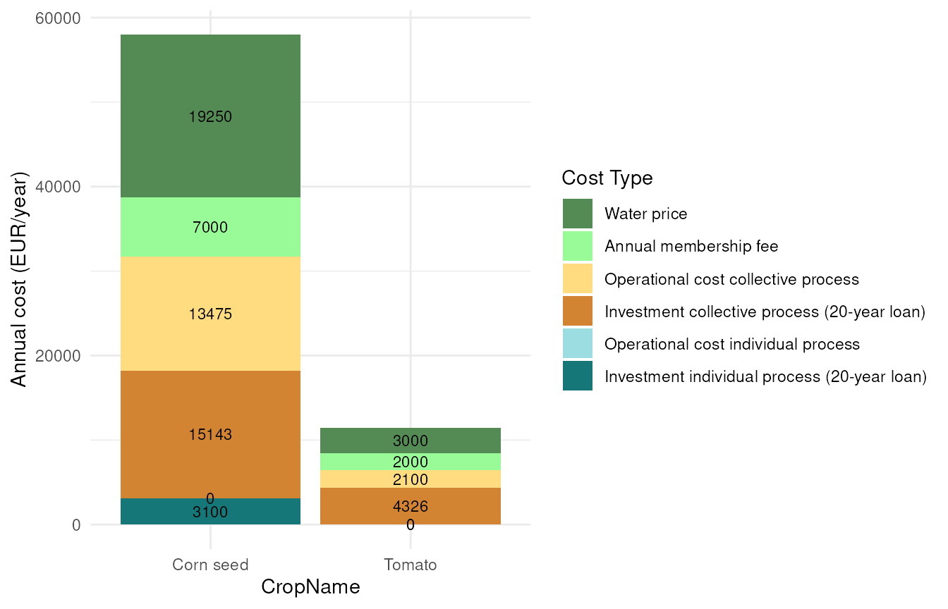

Capex compares their up-front investment:

plots$total_investement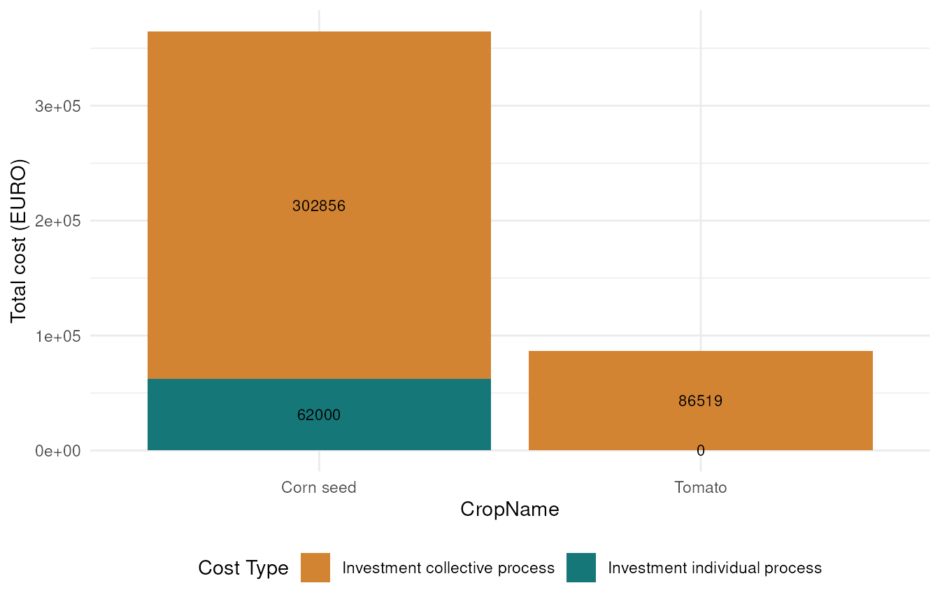

This graph is display only if initialSituation = FALSE, as the initial situation corresponds to the current situation and therefore does not require any investment.

plots$allocation_key
#>   grant  CropName allocation
#> 1   0.5    Tomato     0.1111
#> 2   0.5 Corn seed     0.3889

This allocation key is calculated by default in function collective_treatment_cost, but it can be customised by the user using parameter allocation_key, which is set to NULL by default. This parameter accepts a vector of percentage values of the same size as the number of simulated crops.


crop <- scenario$CropName
allocation_custom <- data.frame(CropName = crop,
                                allocation = c(0.5, 0.5))
run_economic_analysis(
  scenario,
  membership_fee = 200,   
  price_per_m3   = 0.1,   
  grant          = 0,   
  initialSituation = FALSE, 
  allocation_key = allocation_custom # No subvention, collective treatment price 50% for each crop
)
#> $annual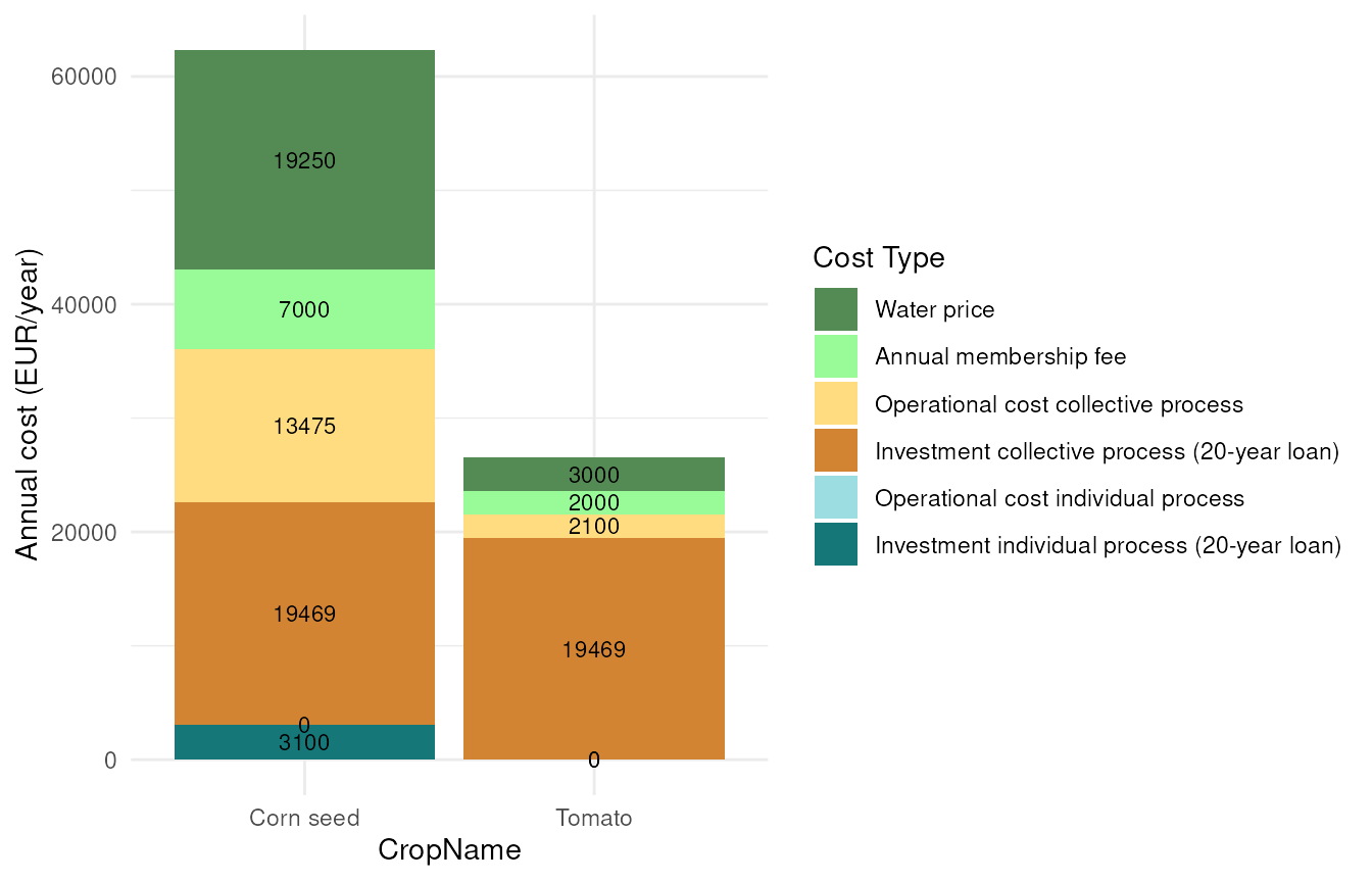

#> 
#> $total_investement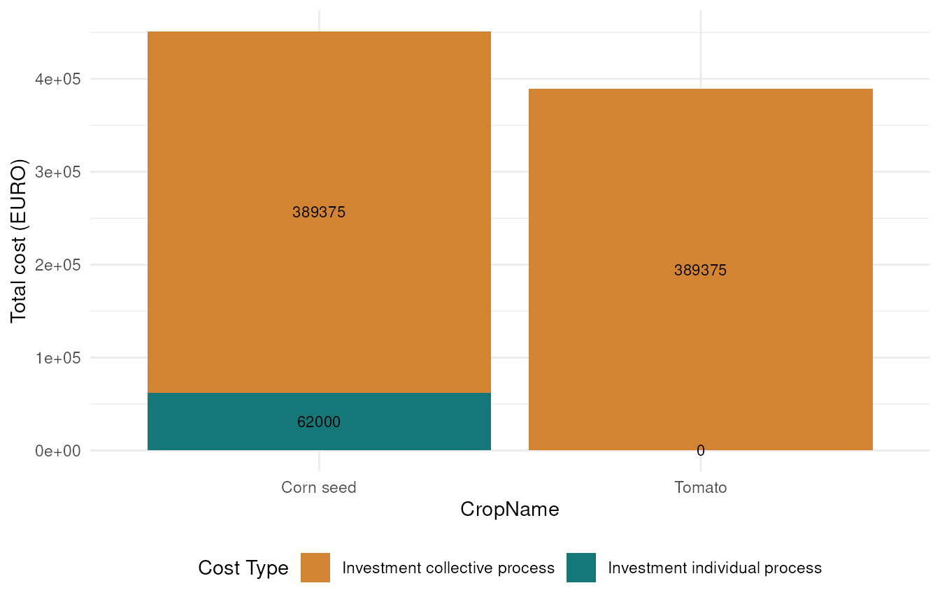

#> 
#> $allocation_key
#>   grant  CropName allocation
#> 1     0    Tomato        0.5
#> 2     0 Corn seed        0.5

Getting the underlying numbers

The run_ function returns only plots. To get the figures behind them, call the costing functions yourself. They expect the scenario to carry its irrigation need first, so run irrigation_need_calculation() before them:

scenario_need <- irrigation_need_calculation(scenario)

water_price <- water_price(scenario = scenario_need,
                          price_per_m3 = 0.01,
                          membership_fee = 200)
supplementary_cost <- process_cost_calculation(scenario = scenario_need,
                                              membership_fee = 200,
                                              charge = 0.1,
                                              initialSituation = FALSE)

Each returns the scenario augmented with cost columns; the added columns are the ones to inspect:

setdiff(names(water_price), names(supplementary_cost))
#> [1] "water_charge"          "annual_membership_fee"

Caveats worth flagging

The situations are modelled asymmetrically. The initial and supplementary process cases do not carry exactly the same cost structure, so read the comparison as orders of magnitude rather than a precise like-for-like tender.

Adapting the cost base

The prices are not hard-coded in the functions – they live in a CSV. To cost a scheme for your own territory, edit data-raw/ambre_barriere_cout.csv (keeping the unit convention), then rebuild the bundled dataset by sourcing data-raw/config_ambre.R. The next run_economic_analysis() will use your numbers. The database and this rebuild step are described in vignette("h-config-ambre", package = "ambre").