
Initial situation VS New scenario
b-initial-vs-new-scenario.RmdThere are many ways to reduce the health risk associated with water reuse. A scheme can be improved by adding a treatment process, introducing an additional field barrier, changing irrigation practices, or modifying exposure conditions.
ambre allows you to compare an initial
situation with a modified scenario on the same
quantitative microbial risk assessment (QMRA) scale. Both scenarios are
simulated with the same Monte Carlo engine, making it easy to evaluate
the effect of a proposed change on pathogen concentrations, infection
risk and DALYs.
New to the pipeline? Read
vignette("a-get-started", package = "ambre") first.
Treatments and field barriers live in one table
ambre does not consider “treatment” and “practices” as
different kinds of thing. Both are just log-reductions
– a number of log10 units of pathogen removed – stored side
by side in one table, config_ambre$treatment$processes. Its
entries are coded by barrier types : Q. for water
quality (treatment processes), E. for on-field
equipment, P. for cultivation and irrigation
practices.
tn <- sort(unique(config_ambre$treatment$processes$TreatmentName))
head(tn, 15)
#>  [1] "E.1 - Automatic irrigation"
#>  [2] "E.1.1 - Micro-sprinkler"
#>  [3] "E.1.2 - Surface drip irrigation"
#>  [4] "E.1.3 - Subsurface drip irrigation"
#>  [5] "E.2 - Mechanised crop maintenance"
#>  [6] "E.3 - Mechanised harvesting"
#>  [7] "E.4 - Signage"
#>  [8] "E.5 - Fences"
#>  [9] "E.7 - Sheet mulching"
#> [10] "E.8 - Personnal Protective Equipement"
#> [11] "P.1 - Non-edilble crop"
#> [12] "P.10 - Rinsing with drinking water"
#> [13] "P.11 - Washing with disinfectant"
#> [14] "P.2 - Distance of 70m"
#> [15] "P.3 - Night-time irrigation"
Each process is characterised by a distribution of pathogen
log-reductions and identified by its TreatmentID. Depending
on the scenario, one or more processes can be added to the existing
treatment train to represent an improvement of the reuse scheme.
How the Excel prepares two trains
The Excel input file describes the initial reuse scheme
InitialProcessName. Additional processes can then be
introduced to build a modified scenario while keeping every other
parameter identical SupplementaryProcessName.
This approach makes it possible to quantify the benefit of a proposed intervention under exactly the same exposure assumptions.
Your input file carries four columns describing the barrier chain:
readxl::read_excel(
  system.file("input_1culture_2pop.xlsx", package = "ambre")
)[, c("STEPtreatmentName", "CollectiveTreatmentName",
      "InitialProcessName", "SupplementaryProcessName")]
#> # A tibble: 2 × 4
#>   STEPtreatmentName      CollectiveTreatmentName InitialProcessName
#>   <chr>                  <chr>                   <chr>
#> 1 Q.1 - Activated Sludge Q.2 - Maturation Pond   Q.6 - Chlorination
#> 2 Q.1 - Activated Sludge Q.2 - Maturation Pond   Q.6 - Chlorination
#> # ℹ 1 more variable: SupplementaryProcessName <chr>
From these, create_scenario() assembles two
candidate trains:
- the initial train – wastewater treatment plant + collective treatment + initial process;
- the supplementary train – wastewater treatment plant + collective treatment + initial process + * supplementary process.
The switch is a single line
run_qmra_initial_situation() and
run_qmra_supplementary_processs() are the same
pipeline. The only difference is one argument passed deep inside them,
update_treatment_scheme(initial_situation = ...), which
decides which train is injected into the config before the
log-reductions are simulated:
-
run_qmra_treatment()usesinitial_situation = TRUE-> the initial train; -
run_qmra_barrier()usesinitial_situation = FALSE-> the supplementary train.
Everything else – inflow, exposure volume, dose, dose-response, DALYs – is computed identically. In particular, only the concentration log-reduction differs between the two runs; the exposure side is unchanged.
Run and overlay the two strategies
plot_comparison_qmra_initial_vs_supplementary_processes()
runs both pipelines on the same input scenario file and pathogen and
returns three side-by-side comparisons – log-reduction, and DALYs – each
a cowplot panel with the initial result on the left and the
supplementary result on the right.
library(dplyr)
scenario_example <- create_scenario(filepath = system.file("input_1culture_2pop.xlsx", package = "ambre"))
regulation_reduction <- config_ambre$regulation$regulation_value |> filter(Country == "France") |>
                          select(-c(Concentration, Country, RegulationID))
regulation_concentration <- config_ambre$regulation$regulation_value |> filter(Country == "France") |>
                        select(-c(Country, RegulationID, Reduction))

comparison <- plot_comparison_qmra_initial_vs_supplementary_processes(
  scenario = scenario_example,
  pathogen = c("Campylobacter jejuni"),
  regulationLog = regulation_reduction,
  regulationConcentration = regulation_concentration
)
names(comparison)
#> [1] "log_reduction" "dalys"
Log-reduction – how much each train removes. This is where the two strategies visibly diverge, because it is the only step that differs.
comparison$log_reduction
#> $Bacteria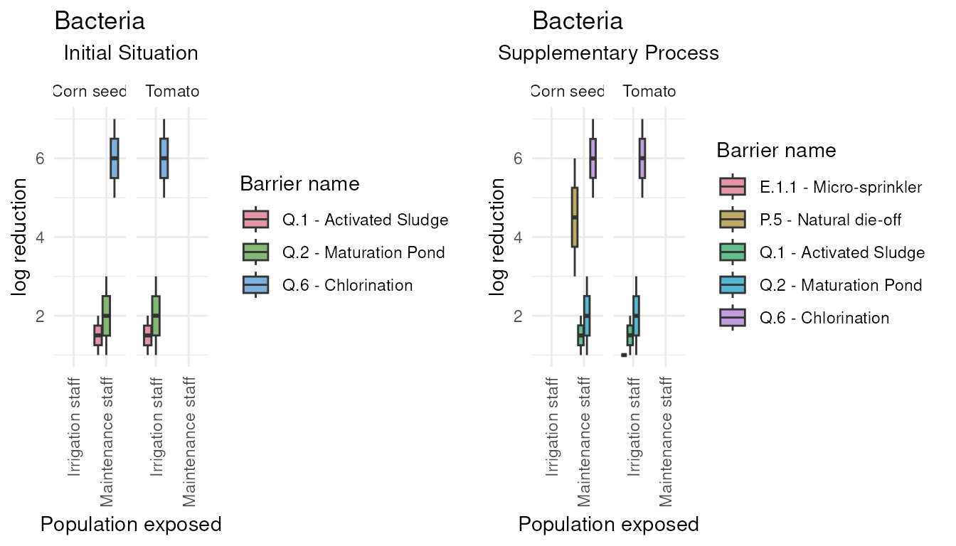
DALYs – the health burden per person per year, both panels sharing the red WHO 1e-6 reference line. Reading the two boxplots against that line tells you whether either strategy – or which one – brings the scheme under the tolerable target.
comparison$dalys
#> $`Campylobacter jejuni`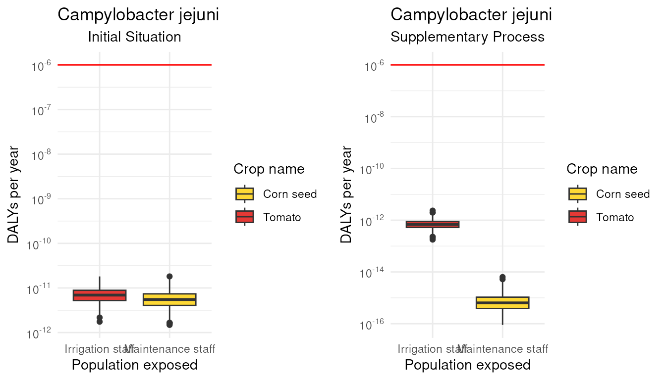
For how to read these ranges and conclude, see
vignette("d-interpreting-risk", package = "ambre").
Scope and current limits
The multi-barrier idea is powerful, but be honest about what the engine credits today:
- Barrier credits add in log space. Within a train, the log-reductions of the successive barriers are summed. Combining a modest treatment with a good field practice can reach the target without ever-heavier treatment – exactly the argument behind the WHO multi-barrier guidance and EU Regulation 2020/741 (which lets a scheme meet a reclaimed-water class through additional barriers rather than more treatment).
-
Some data relating to barriers vary depending on the route
of exposure, the crop and agricultural practices
config_ambre$treatmentcontains the tablesbarriere_path,barriere_specificandbarriere_decay. These are used to update the source databaseconfig_ambre$processesaccording to the simulated scenario; with functionretrieve_specific_barrier
To see the underlying database for yourself, read
vignette("h-config-ambre", package = "ambre").